Examples
Getting Started
Here, we’ll look up the reddening at a number of different locations on the sky. We specify coordinates on the sky using astropy.coordinates.SkyCoord objects. This allows us a great deal of flexibility in how we specify sky coordinates. We can use different coordinate frames (e.g., Galactic, equatorial, ecliptic), different units (e.g., degrees, radians, hour angles), and either scalar or vector input.
For our first example, let’s load the Schlegel, Finkbeiner & Davis (1998) – or “SFD” – dust reddening map, and then query the reddening at one location on the sky:
from __future__ import print_function
from astropy.coordinates import SkyCoord
from dustmaps.sfd import SFDQuery

coords = SkyCoord('12h30m25.3s', '15d15m58.1s', frame='icrs')
sfd = SFDQuery()
ebv = sfd(coords)

print('E(B-V) = {:.3f} mag'.format(ebv))

>>> E(B-V) = 0.030 mag
A couple of things to note here:
In this example, we used
from __future__ import print_functionin order to ensure compatibility with both Python 2 and 3.Above, we used the ICRS coordinate system, by specifying
frame='icrs'.SFDQueryreturns reddening in a unit that is similar to magnitudes of E(B-V). However, care should be taken: a unit of SFD reddening is not quite equivalent to a magnitude of E(B-V). The way to correctly convert SFD units to extinction in various broadband filters is to use the conversions in Table 6 of Schlafly & Finkbeiner (2011).
We can query the other maps in the dustmaps package with only minor
modification to the above code. For example, here’s how we would query the
Planck Collaboration (2013) dust map:
from __future__ import print_function
from astropy.coordinates import SkyCoord
from dustmaps.planck import PlanckQuery

coords = SkyCoord('12h30m25.3s', '15d15m58.1s', frame='icrs')
planck = PlanckQuery()
ebv = planck(coords)

print('E(B-V) = {:.3f} mag'.format(ebv))

>>> E(B-V) = 0.035 mag
Querying Reddening at an Array of Coordinates
We can also query an array of coordinates, as follows:
from __future__ import print_function
import numpy as np
from astropy.coordinates import SkyCoord
from dustmaps.planck import PlanckQuery
from dustmaps.sfd import SFDQuery

l = np.array([0., 90., 180.])
b = np.array([15., 0., -15.])

coords = SkyCoord(l, b, unit='deg', frame='galactic')

planck = PlanckQuery()
planck(coords)
>>> array([ 0.50170666,  1.62469053,  0.29259142])

sfd = SFDQuery()
sfd(coords)
>>> array([ 0.55669367,  2.60569382,  0.37351534], dtype=float32)
The input need not be a flat array. It can have any shape – the shape of the output will match the shape of the input:
from __future__ import print_function
import numpy as np
from astropy.coordinates import SkyCoord
from dustmaps.planck import PlanckQuery

l = np.linspace(0., 180., 12)
b = np.zeros(12, dtype='f8')
l.shape = (3, 4)
b.shape = (3, 4)

coords = SkyCoord(l, b, unit='deg', frame='galactic')

planck = PlanckQuery()

ebv = planck(coords)

print(ebv)
>>> [[ 315.52438354   28.11778831   23.53047562   20.72829247]
     [   2.20861101   15.68559361    1.46233201    1.70338535]
     [   0.94013882    1.11140835    0.38023439    0.81017196]]

print(ebv.shape)
>>> (3, 4)
Querying 3D Reddening Maps
When querying a 3D dust map, there are two slight complications:
There is an extra axis – distance – to care about.
Many 3D dust maps are probabilistic, so we need to specify whether we want the median reddening, mean reddening, a random sample of the reddening, etc.
Let’s see how this works out with the “Bayestar” 2019 3D dust map of Green et al. (2019). The DECaPS 3D dust map from Zucker, Saydjari, and Speagle et al. (2025) (complementing Bayestar in the southern Galactic plane) can be queried in a similar manner, with a few key differences outlined later on in the examples.
How Distances are Handled
If we don’t provide distances in our input, dustmaps will assume we want dust
reddening along the entire line of sight.
from __future__ import print_function
from astropy.coordinates import SkyCoord
from dustmaps.bayestar import BayestarQuery

coords = SkyCoord(180., 0., unit='deg', frame='galactic')

bayestar = BayestarQuery(max_samples=2, version='bayestar2019')

E = bayestar(coords, mode='random_sample')

print(E)
>>> [0.         0.         0.         0.         0.         0.
     0.         0.         0.         0.         0.         0.
     0.         0.         0.         0.         0.         0.04
     0.04       0.04       0.04       0.04       0.04       0.04
     0.04       0.05       0.05       0.05       0.07       0.09
     0.09       0.09       0.09999999 0.09999999 0.09999999 0.11
     0.11       0.11       0.11       0.12       0.12       0.12
     0.12       0.12       0.14       0.14       0.16       0.17999999
     0.19       0.19999999 0.21       0.21       0.22       0.22999999
     0.22999999 0.26999998 0.26999998 0.57       0.59       0.59
     0.59       0.68       0.69       0.7        0.71       0.77
     0.78       0.81       0.82       0.82       0.83       0.85999995
     0.87       0.98999995 0.98999995 1.02       1.02       1.03
     1.09       1.11       1.11       1.11       1.11       1.11
     1.11       1.11       1.11       1.11       1.11       1.11
     1.11       1.11       1.11       1.11       1.11       1.11
     1.12       1.12       1.12       1.12       1.12       1.12
     1.12       1.12       1.12       1.12       1.12       1.12
     1.12       1.12       1.12       1.12       1.12       1.12
     1.12       1.12       1.12       1.12       1.12       1.12]
Here, the Bayestar map has given us a single random sample of the cumulative dust reddening along the entire line of sight – that is, to a set of distances. To see what those distances are, we can call:
bayestar.distances
>>> <Quantity [ 0.06309573,  0.06683439,  0.07079458,  0.07498942,
                0.07943282,  0.08413951,  0.08912509,  0.09440609,
                0.1       ,  0.10592537,  0.11220185,  0.11885022,
                0.12589254,  0.13335214,  0.14125375,  0.14962357,
                0.15848932,  0.1678804 ,  0.17782794,  0.18836491,
                0.19952623,  0.2113489 ,  0.22387211,  0.23713737,
                0.25118864,  0.26607251,  0.28183829,  0.29853826,
                0.31622777,  0.33496544,  0.35481339,  0.3758374 ,
                0.39810717,  0.4216965 ,  0.44668359,  0.47315126,
                0.50118723,  0.53088444,  0.56234133,  0.59566214,
                0.63095734,  0.66834392,  0.70794578,  0.74989421,
                0.79432823,  0.84139514,  0.89125094,  0.94406088,
                1.        ,  1.05925373,  1.12201845,  1.18850223,
                1.25892541,  1.33352143,  1.41253754,  1.49623566,
                1.58489319,  1.67880402,  1.77827941,  1.88364909,
                1.99526231,  2.11348904,  2.23872114,  2.37137371,
                2.51188643,  2.66072506,  2.81838293,  2.98538262,
                3.16227766,  3.34965439,  3.54813389,  3.75837404,
                3.98107171,  4.21696503,  4.46683592,  4.73151259,
                5.01187234,  5.30884444,  5.62341325,  5.95662144,
                6.30957344,  6.68343918,  7.07945784,  7.49894209,
                7.94328235,  8.41395142,  8.91250938,  9.44060876,
               10.        , 10.59253725, 11.22018454, 11.88502227,
               12.58925412, 13.33521432, 14.12537545, 14.96235656,
               15.84893192, 16.78804018, 17.7827941 , 18.83649089,
               19.95262315, 21.1348904 , 22.38721139, 23.71373706,
               25.11886432, 26.6072506 , 28.18382931, 29.85382619,
               31.6227766 , 33.49654392, 35.48133892, 37.58374043,
               39.81071706, 42.16965034, 44.66835922, 47.3151259 ,
               50.11872336, 53.08844442, 56.23413252, 59.56621435] kpc>
The return type is an astropy.unit.Quantity instance, which keeps track of units.
If we provide Bayestar or DECaPS with distances, then it will do the distance interpolation for us, returning the cumulative dust reddening out to specific distances:
import astropy.units as units

coords = SkyCoord(180.*units.deg, 0.*units.deg,
                  distance=500.*units.pc, frame='galactic')
E = bayestar(coords, mode='median')

print(E)
>>> 0.105
Because we have explicitly told Bayestar what distance to evaluate the map at, it returns only a single value.
How Probability is Handled
The Bayestar and DECaPS 3D dust maps are probabilistic, meaning that they store random samples
of how dust reddening could increase along each sightline. Sometimes we might be
interested in the median reddening to a given point in space, or we might want
to have all the samples of reddening out to that point. We specify how we want
to deal with the probabilistic nature of the map by providing the keyword
argument mode to dustmaps.bayestar.BayestarQuery.__call__.
For example, if we want all the reddening samples, we invoke:
l = np.array([30.,  60., 90.]) * units.deg
b = np.array([10., -10., 15.]) * units.deg
d = np.array([1.5,  0.3, 4.0]) * units.kpc

coords = SkyCoord(l, b, distance=d, frame='galactic')

E = bayestar(coords, mode='samples')

print(E.shape)  # (# of coordinates, # of samples)
>>> (3, 2)

print(E)
>>> [[0.26999998 0.29999998]  # Two samples at the first coordinate
...  [0.         0.01      ]  # Two samples at the second coordinate
...  [0.09999999 0.08      ]] # Two samples at the third coordinate
If we instead ask for the mean reddening, the shape of the output is different:
E = bayestar(coords, mode='mean')

print(E.shape)  # (# of coordinates)
>>> (3,)

print(E)
>>> [0.28499997 0.005      0.09      ]
The only axis is for the different coordinates, because we have reduced the samples axis by taking the mean.
In general, the shape of the output from the Bayestar and DECaPS maps is:
(coordinate, distance, sample)
where any of the axes can be missing (e.g., if only one coordinate was specified, if distances were provided, or if the median reddening was requested).
Percentiles are handled in much the same way as samples. In the following query, we request the 16th, 50th, and 84th percentiles of reddening at each coordinate, using the same coordinates as we generated in the previous example:
E = bayestar(coords, mode='percentile', pct=[16., 50., 84.])

print(E)
>>> [[0.27479998  0.28499998  0.29519998]  # Percentiles at 1st coordinate
     [0.0016      0.005       0.0084    ]  # Percentiles at 2nd coordinate
     [0.0832      0.09        0.09679999]] # Percentiles at 3rd coordinate
We can also pass a single percentile:
E = bayestar(coords, mode='percentile', pct=25.)

print(E)
>>> [0.27749997  0.0025      0.08499999]  # 25th percentile at 3 coordinates
Getting Quality Assurance Flags from the Bayestar and DECaPS Dust Maps
For the Bayestar and DECaPS dust maps, one can retrieve QA flags by providing the keyword
argument return_flags=True:
E, flags = bayestar(coords, mode='median', return_flags=True)

print(flags.dtype)
>>> [('converged', '?'), ('reliable_dist', '?')]

print(flags['converged'])  # Whether or not fit converged in each pixel
>>> [ True  True  True]

# Whether or not map is reliable at requested distances
print(flags['reliable_dist'])
>>> [ True False  True]
DECaPS shares the same quality flags as Bayestar, but includes one additional flag, called “infilled”, which indicates whether the pixel needed to be infilled due to an insufficient number of stars:
>>> [('converged', '?'), ('infilled', '?'), ('reliable_dist', '?')]
If the coordinates do not include distances, then instead of
'reliable_dist', the query will return the minimum and maximum reliable
distance moduli of the map in each requested coordinate:
l = np.array([30.,  60., 90.]) * units.deg
b = np.array([10., -10., 15.]) * units.deg

coords = SkyCoord(l, b, frame='galactic')

E, flags = bayestar(coords, mode='median', return_flags=True)

print(flags['min_reliable_distmod'])
>>> [ 7.5968404  7.9513497  6.7628193]

print(flags['max_reliable_distmod'])
>>> [14.584786 14.536094 14.613377]
We can see from the above that in the previous example, the reason the second coordinate was labeled unreliable was because the requested distance (300 pc) was closer than a distance modulus of 7.95 (corresponding to ~389 pc).
Combining the Bayestar and DECaPS 3D Dust Maps
The DECaPS map can largely be queried in a similar manner to the Bayestar map. However, due to the increased angular resolution of the DECaPS map (approximately 1′), the size of the data products is significantly larger. To accommodate users with limited storage, the dustmaps package provides a few additional options.
First, users may choose to download only the mean map (~8 GB), which is significantly smaller than the full dataset containing both the mean and samples (~33 GB). If only the mean map is downloaded, an additional argument must be specified (mean_only=True) that precludes querying in any other mode (e.g. random sample, etc. )
from dustmaps.decaps import DECaPSQuery
decaps = DECaPSQuery(mean_only=True)
By default, the DECaPSQuery class loads the full map into memory. For lightweight usage, dustmaps also provides DECaPSQueryLite, which uses memory mapping to avoid loading the full dataset into RAM. This is ideal for small queries:
from dustmaps.decaps import DECaPSQueryLite
decapslite = DECaPSQueryLite()
To combine the Bayestar and DECaPS 3D dust maps, users should query Bayestar for regions north of declination −30°, and DECaPS for regions south of declination −30°, taking advantage of each map’s sky coverage. For example, we can generate a few dozen random coordinates in the Galactic plane, filter them by declination, and query the appropriate map based on each coordinate’s position:
import numpy as np
from astropy.coordinates import SkyCoord
from astropy import units

# Generate random coordinates in the plane
n_coords = 50
l = np.random.uniform(0, 360, n_coords)
b = np.random.uniform(-10, 10, n_coords)

gal_coords = SkyCoord(l=l*units.deg, b=b*units.deg, distance=3*units.kpc, frame='galactic')

# Filter based on declination
mask_north = gal_coords.icrs.dec.deg > -30
mask_south = gal_coords.icrs.dec.deg <= -30

# Query both maps
ebv_bs = 0.883 * bayestar(gal_coords[mask_north], mode='random_sample')
ebv_decaps = decapslite(gal_coords[mask_south], mode='random_sample')

# Compile reddening results
ebv_compiled = np.empty((n_coords))
ebv_compiled[mask_north] = ebv_bs
ebv_compiled[mask_south] = ebv_decaps

print(ebv_compiled)
>>> [0.66225004 1.43870151 0.37085998 0.48639923 0.99045843 0.44150001
 0.16003418 0.45948145 0.21081543 0.2649     0.10596    0.18994141
 0.36010742 0.32671002 0.44150001 1.25460923 0.70639998 1.26343918
 0.57394999 0.04415    0.83002001 1.64257812 0.53054923 0.27373001
 1.28992915 0.09713    0.32671002 0.81385845 0.32671002 0.21191999
 0.58278    1.52246094 0.49597847 0.26564923 0.83885002 2.88815928
 0.22075    1.46191406 0.12362    0.93672919 0.2767269  0.89332843
 0.52096999 0.16003418 0.88449842 0.13171387 0.49448001 0.25
 0.24724001 2.921875  ]
The DECaPS map reports reddening directly in units of E(B−V), while the Bayestar19 map uses arbitrary units. To convert Bayestar19 to E(B−V), we use the relation E(B−V) = 0.883 × E_Bayestar19. This conversion factor is based on Equation 30 from Green et al. (2019), which gives E(g−r) = 0.901 × E_Bayestar19, combined with the relation E(B−V) = 0.98 × E(g−r) from Schlafly & Finkbeiner (2011).
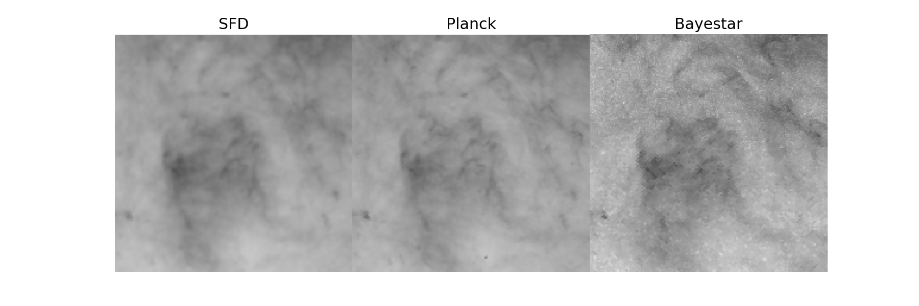
Plotting the Dust Maps
We’ll finish by plotting a comparison of the SFD, Planck Collaboration, Bayestar, and DECaPS dust maps. First, we’ll import the necessary modules:
from __future__ import print_function

import matplotlib
import matplotlib.pyplot as plt
import numpy as np

import astropy.units as units
from astropy.coordinates import SkyCoord

from dustmaps.sfd import SFDQuery
from dustmaps.planck import PlanckQuery
from dustmaps.bayestar import BayestarQuery
from dustmaps.decaps import DECaPSQuery
Next, we’ll set up a grid of coordinates to plot, centered on a small region of the sky toward the Pipe Nebula, where the Bayestar and DECaPS dust maps have overlapping coverage (near declination = -30°):
l0, b0 = (3, 5)
l = np.arange(l0 - 2., l0 + 2., 0.01)
b = np.arange(b0 - 2., b0 + 2., 0.01)
l, b = np.meshgrid(l, b)
coords = SkyCoord(l*units.deg, b*units.deg,distance=5*units.kpc,frame='galactic')
Then, we’ll load up and query four different dust maps:
sfd = SFDQuery()
Av_sfd = 2.74 * sfd(coords)

planck = PlanckQuery()
Av_planck = 3.1 * planck(coords)

bayestar = BayestarQuery()
Av_bayestar = 2.74 * bayestar(coords, mode='mean')

decaps = DECaPSQuery(mean_only=True)
Av_decaps = 3.32 * decaps(coords, mode='mean')
We’ve assumed \(R_V = 3.1\), and used the coefficient from Table 6 of Schlafly & Finkbeiner (2011) to convert SFD and Bayestar reddenings to magnitudes of \(A_V\). We assumed \(R_V = 3.32\) from Schlafly et al. (2016) to convert DECaPS.
Finally, we create the figure using matplotlib:
fig = plt.figure(figsize=(16,4), dpi=150)

for k,(Av,title) in enumerate([(Av_sfd, 'SFD'),
                               (Av_planck, 'Planck'),
                               (Av_bayestar, 'Bayestar19'),
                               (Av_decaps,'DECaPS')]):
    ax = fig.add_subplot(1,4,k+1)
    ax.imshow(
        Av[:, ::-1],
        vmin=0.,
        vmax=10,
        origin='lower',
        interpolation='nearest',
        cmap='binary',
        aspect='equal'
    )
    ax.axis('off')
    ax.set_title(title)

fig.subplots_adjust(wspace=0., hspace=0.)
plt.savefig('comparison.png', dpi=300)
Here’s the result:
Querying the web server
Some of the maps included in this package are large, and can take up a lot of memory, or be slow to load. To make it easier to work with these maps, some of them are available to query over the internet. As of now, the following maps can be queried remotely:
Bayestar (all versions)
SFD
The API for querying these maps remotely is almost identical to the API for local queries. For example, the following code queries SFD remotely:
from __future__ import print_function
from astropy.coordinates import SkyCoord
from dustmaps.sfd import SFDWebQuery

l = [180., 160.]
b = [30., 45.]
coords = SkyCoord(l, b, unit='deg', frame='galactic')
sfd = SFDWebQuery()
ebv = sfd(coords)

print(ebv)

>>> [0.04704102 0.02022794]
The following example queries the Bayestar2019 dust map remotely. The web interface takes the same arguments as the local interface:
import astropy.units as u
from dustmaps.bayestar import BayestarWebQuery

l = [90., 150., 35.] * u.deg
b = [10., 12., -25.] * u.deg
d = [500., 3500., 1000.] * u.pc
coords = SkyCoord(l, b, distance=d, frame='galactic')

q = BayestarWebQuery(version='bayestar2019')
E = q(coords, mode='median')

print(E)

>>> [0.13       0.63       0.09999999]
The query_gal() and query_equ() convenience functions also
work with web queries. Continuing from the previous example,
E = q.query_gal([120., 125.], [-5., -10.],
                d=[1.5, 1.3],
                mode='random_sample')
print(E)

>>> [0.32 0.24]
Please take it easy on our web server. If you want to query multiple coordinates, then bundle them up into one query. If you want to query a very large number of coordinates, consider downloading the maps and querying them locally instead.